ctffind4
CTFFIND 4
June 2017
What's new?
|
 |
ChangeLog
4.1.14
- bug fixes (memory, equiphase averaging)
- bug fixes from David Mastronarde (fixed/known phase shift)
4.1.13
- EPA bug fixed (affected 4.1.12 only)
4.1.12
- diagnostic image includes radial "equi-phase" average of experimental spectrum in bottom right quadrant
- new "equi-phase averaging" (EPA) code will probably replace zero-counting eventually
- bug fix (affected diagnostics for all 4.x): at very high resolution, Cs dominates and the phase aberration decreases
- bug fix (affected 4.1.11): fitting was only done up to 5Å
- slow, exhaustive search is no longer the default (since astigmatism-related bugs appear fixed)
- Number of OpenMP threads defaults to 1 and can be set by:
- using interactive user input (under expert options)
- using the -j command-line option (overrides interactive user input)
- printout timing information
4.1.11
- speed-ups from David Mastronarde, including OpenMP threading of the exhaustive search
- score is now a normalized cross-correlation coefficient (David Mastronarde)
4.1.10
- astimatism-related bug fixes from David Mastronarde
4.1.9
- FRC is between a re-normalized version of the amplitude spectrum, to emphasize phase of the Thon rings over their relative amplitudes
- tweaked criteria for "fit resolution"
- tweaked FRC computation
- astigmatism restraint is off by default
- fixed bug affecting astigmatism
- tweaked background subtraction (thanks Niko!) - helps with noisy VPP spectra
Changes from 4.1.5 to 4.1.8:
- slower search (a la 4.0) is now default, because of reports the faster 1D search was significantly less accurate (thanks Rado Danev & Tim Grant). This is easy to change via the UI to get faster fits.
- TIF files can be read on input
- input movies need not be gain corrected, separate gain file can be given as input (can be DM format) (via expert option)
- input movies need not be corrected for anisotropic magnification (via expert option)
- can be built on MacOS (using brew tools). Better conformance to standard C++.
New in version 4.1:
- Faster than version 4.0
- Option to fix the amount and angle of astigmatism
- Resamples data when the input pixel size is too small (can be switched off using expert options)
- Warns if CTF aliasing is detected
- Improved diagnostic 1D plots
New in version 4.0.16: command-line option --fast to skip some extra statistics, spend less time on diagnostic output and save compute time; improved background subtraction; more low-level optimisations - should be significantly faster; background subtraction more robust, tested on wider range of micrographs
New in version 4.0.10: find phase shift due to phase plate, new command-line options to give amplitude spectra rather than images as input, buildable using GNU compilers (>=4.9.1), support for MRC mode 6 files, bug fixes
New in version 4.0.8: improved contrast in diagnostic image, improved estimate of resolution at which Thon rings were detected, minor bug fixes
Where can I download it?
Please go to the ctffind page.
Why is it faster?
Mainly because the astigmatism azimuth angle is estimated separately from defocus parameters, making the search & refinement 2- rather than 3-dimensional.
Also, many parts of the code were optimized for speed.
In version 4.1 onwards, the initial search for defocus is done on the 1D radial average of the amplitude spectrum rather than on the 2D spectrum (h/t Kai Zhang), unless very large astigmatism is expected. In version 4.1.8 onwards, this accelerated 1D search is not default anymore because of reports that it yielded slightly less accurate results (h/t Rado Danev & Tim Grant).
Does it do exactly the same thing as CTFFIND 3?
No, and it doesn't give exactly the same results, but the results should be very, very similar. Below are some of main differences in processing between CTFFIND 3 and CTFFIND 4:
- The astigmatism angle is estimated separately from the defocus parameters
- Rather than estimating the micrograph power spectrum by averaging spectra from many tiles, a single large Fourier transform of the whole micrograph is computed and then downsampled for CTF fitting.
- All areas of the micrograph are used for power spectrum estimation
- Micrograph edges are "tapered" on input, a la MRC.
- Amplitudes, rather than intensities, are computed and fit with a CTF model.
Other aspects of the algorithm have not changed from CTFFIND 3 to CTFFIND 4.
Should I switch from CTFFIND 3 to CTFFIND 4?
If you are working on micrographs which were collected on photographic film and scanned in, you should probably stick with CTFFIND 3, because micrograph features such as film labels or scratches may throw CTFFIND 4 off, whereas CTFFIND 3 should ignore them. Otherwise, if you are working on images from CCDs or direct detectors, you should switch to CTFFIND 4: it is significantly faster and may give better estimates of the power spectrum because it will not discard any part of the micrograph.
Should I use CTFFIND on unaligned movie frames, or on aligned and averaged frames?
It is worth trying both options on a few typical movies for your dataset first. Estimating from movie frames is much slower but sometimes gives improved Thon rings, especially in the "water ring" (around 3.6 Angstroms), though this can be at the expense of Thon rings at lower resolutions.
Also, if you think there may be significant errors in your alignment of the movie frames, it may be beneficial to give the unaligned frames as input to CTFFIND. If however you are confident in your frame alignment, giving the aligned average as input should give better results when estimating CTF parameters from protein complexes and will run much faster.
When processing stacks of movie frames, you have to chose how many frames should be averaged together (phases and amplitudes) in groups before the amplitude spectra are averaged together. A good starting point is to average ~ 4.0e/A2 worth of frames, based on the work of McMullan & Henderson (Ultramicroscopy, 2015).
Dependencies for ctffind_plot_results.sh script
This scripts requires
- pdftk
- gnuplot >= 4.6, with pdfcairo terminal enabled
What is plotted by the ctffind_plot_results.sh script?
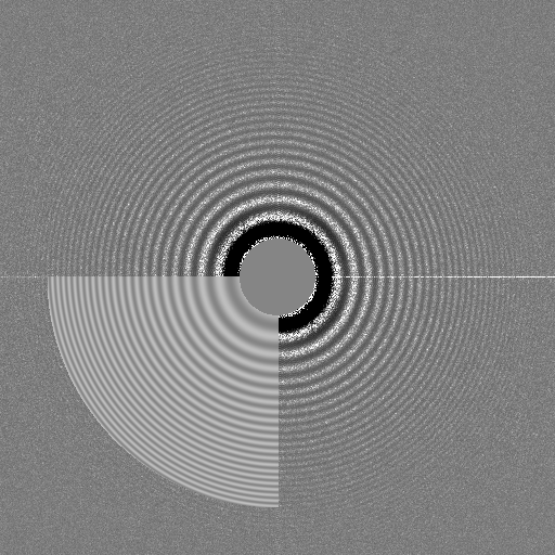
Here is an example of the output from the script:
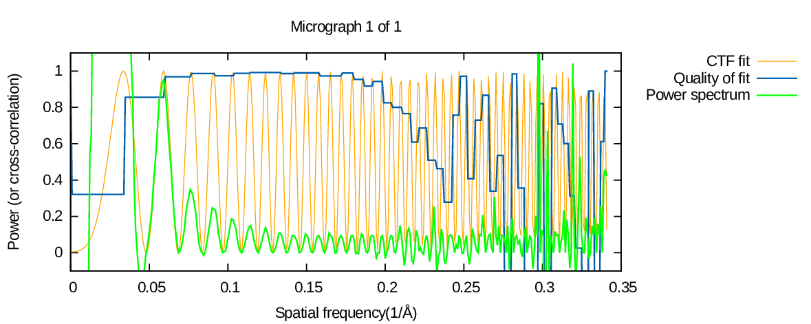
Experimental power spectrum - green line
The green line is a 1D average of the experimental power spectrum obtained from the micrograph. It is computed by taking into account astigmatism. Also, it is normalised to optimise visualisation in the plot:
- The minima of the oscillations are set to 0.0
- Values are normalised such that the second peak of the power spectrum (in this case at around 0.06) is at 0.95
- For spatial frequencies at which the power spectrum maxima are less than 0.1, values are normalised such that the values at estimated maxima positions are 0.1. This means that spatial frequencies at which no CTF rings were present in the power spectrum or at which the CTF estimation was wrong will end up with very noisy-looking 1D spectra.
One consequence of all these normalisation steps is that you should not use this 1D profile to estimate anything quantitative about, say, envelope functions of the microscope.
CTF fit - orange line
The orange line is a 1D average of the 2D theoretical CTF which was fit to the power spectrum. The 1D averaging is done taking astigmatism into account.
Quality of fit - blue line
The blue line plots a measure of the quality of fit between the theoretical CTF (orange) and the experimental power spectrum (green). The quality of fit is calculated once per "cycle" of the squared CTF - the interval from one maximum to the next (in CTFFIND 4.0.x) or over a moving window (in CTFFIND 4.1.x). This estimate is computed as a normalised cross-correlation between the 1D profile of the experimental power spectrum and the 1D profile of the fit CTF.
How does ctffind estimate the highest spacing to which CTF rings were fit successfully?
This value is in the 6th column of the summary output .txt file. It is estimated as the last spatial frequency at which the quality of fit measure is still above 0.5 (0.2 in versions 4.0.x). This threshold was chosen heuristically. Please take this estimate with a pinch of salt.
A word of caution about the estimated CTF fit resolution
This estimate can be very noisy and error-prone. Also, even in cases when it is "well behaved", it may not accurately reflect the quality of your data. Consider the output below, obtained from a dose-fractionated exposure:
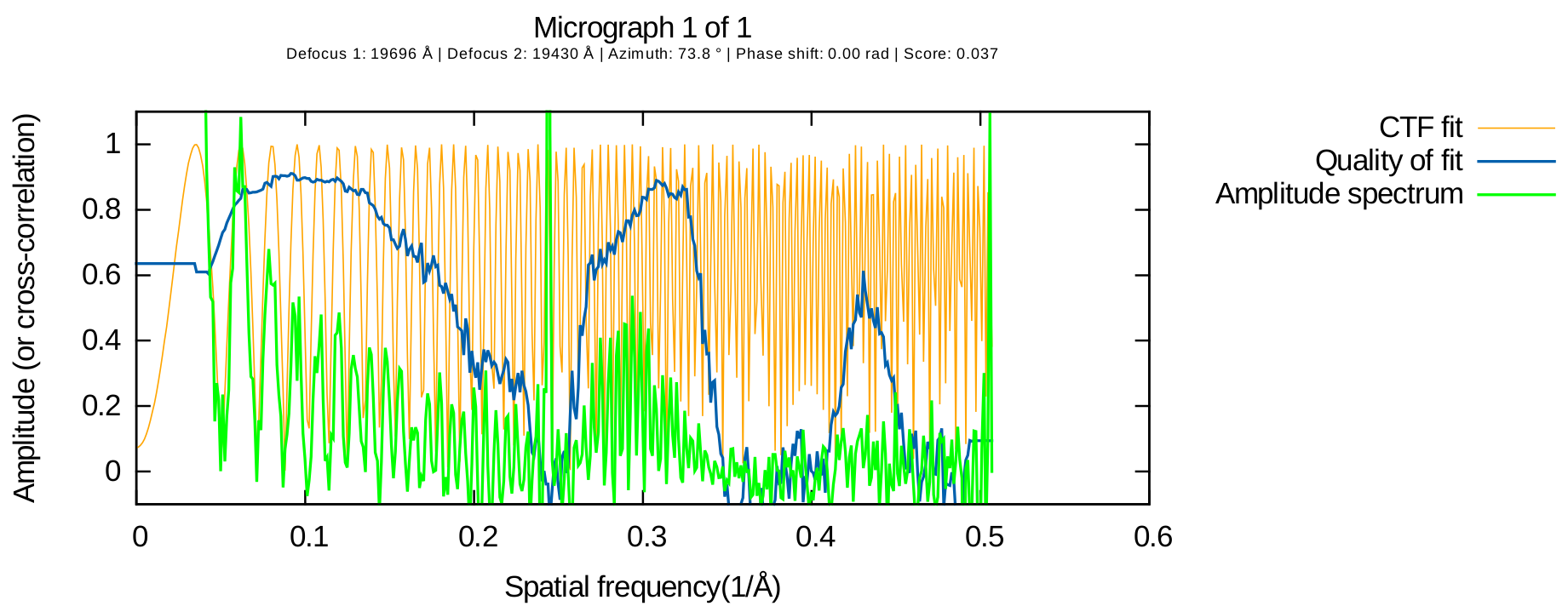
In this case, the reported resolution of the fit was 5.3 Angstrom, though it is obvious that the water ring (around 3.6 Angstroms) had strong Thon rings which were fit successfully.
Running ctffind4 from Relion
To use ctffind4 from Relion 1.3, you need to supply ctffind with the --old-school-input command-line flag. You also need to surround the whole command with double quotes. Here is a simplified example from the command line:
--ctffind3_exe "/lmb/home/tmartin/programs/ctffind-4.0.9-linux64/ctffind --omp-num-threads 1 --old-school-input" Or from the Relion GUI, replace the executable with:
"/lmb/home/tmartin/programs/ctffind-4.0.9-linux64/ctffind --omp-num-threads 1 --old-school-input"
Running from Relion, a warning
The meaning of dAst has changed slightly since previous releases of ctffind. The meaning of 0.0 for this value in ctffind3 was not well documented. It caused ctffind3 (and ctffind <= 4.0.8) to not impose any restraint on the level of astigmatism. This runs counter intuition I believe, since setting this to 0.0 might be expected to mean that we don't want to allow any/much astigmatism.
So I changed this. Now, if the user gives 0.0<=dAst<=10.0 (now called "expected/tolerated astigmatism" in ctffind4), there will be a very strong restraint on astigmatism. To switch off the restraint altogether, the user must set this value to something negative.
The default suggested by ctffind4 is 100.0A, which gives a soft restraint on astigmatism. I have already discussed this with Sjors and the next release of Relion will also use 100.0A as a default. I recommend you do this yourself in the meantime. Versions 4.0.13 and above, when running in --old-school-input mode, treat dAst=0.0 the way ctffind3 does.
Giving amplitude spectra as inputs
Rather than letting ctffind compute them from input micrographs, you can give your own amplitude spectra as inputs to the program. To do this, give --amplitude-spectrum-input at the command line. If you want to give amplitude spectra from which you have already subtracted the background (i.e. you just want ctffind to do CTF fitting, no processing of the spectra themselves), use option --filtered-amplitude-spectrum-input.
OpenMP threading (versions 4.0.x only)
On most systems, the program will use as many OpenMP threads as are available. You can control how many threads are available using standard OpenMP means,
such as setting the environment variable OMP_NUM_THREADS. In addition, you can use the command-line option --omp-num-threads=N or --omp-num-threads N to limit the program to N threads maximum.
Compiling from source (versions 4.0.x)
GNU-style configure & make scripts are provided. We recommend linking against Intel's MKL for faster Fourier transforms.
Here is an example of typical build commands:
mkdir build
cd build
../configure --enable-static --disable-debug --enable-optimisations --enable-openmp FC=gfortran F77=gfortran
make
Compiling from source (versions 4.1.x)
Please refer to the included README file.
Other tips
- Once you have run ctffind on a few representative micrographs, tweak the min and max resolutions for fitting:
- Increase the minimum resolution to "just before" the first zero of the CTF. Despite our best efforts, there are often cases where background subtraction does not work perfectly, and the fit can be improved by ignoring the very low frequencies
- Increase the maximum resolution to approximately where you can see Thon rings in the experimental spectrum and/or where ctffind reports detecting rings. If you are using data up to 8A but rings are visible to ~5A, you are probably not getting as accurate a defoucs estimate as you could get
- Choose a pixel size such that the last visible/fit Thon rings are close to Nyquist. If your pixel size is ~1A but your rings only go up to, say, 5A, you may wish to resample your micrographs to a pixel size of 2A for CTF estimation. This will make CTF estimation faster and may even help with accuracy. This is done automatically by ctffind versions > 4.1.
Author
CTFFIND 4 was written by Alexis Rohou. It started as a rewrite of CTFFIND 3, written by Nikolaus Grigorieff, though it now has a number of additional features.
Bug reports, questions
Please direct requests for help and bug reports to the Grigorieff lab forum: http://grigoriefflab.janelia.org/ctf/forum.
