Zeiss Scanner
Entered On
Type of Procedure
Short Description
Signing Up
You can sign up to reserve time on the Zeiss scanner on this page.- Each person can only sign up for ONE session of up to 6 hours (e.g., 8am-2pm, 2pm-8pm). You can sign up for your next session as soon as your first session is finished.
- If you don't show up by 30 minutes after your session starts, you lose your time. Anyone else can use it.
- If you can not make your session, please delete it! Be nice--let other people know.
- You may continue to scan if no one signs up for the session right after your session.
- It is your responsibility to move your scanned data somewhere other than 'Temp'. The files there could be deleted without warning!
Logging on
- Login as 'emuser' with the usual password
- Start "HyperTerminal" by clicking Start -> Programs -> PhotoScan -> Controller HyperTerminal
- Turn on Scanner and wait until self test is finished and shows OK
- If self test failed, record the error message from HyperTerminal to the log book, and
- Turn off scanner, wait for a minute, turn it back on again.
- After Self Test OK, start PhotoScan software. Pay attention to the green histogram like button "Normalize CCD" button (see below); it should be green and one can click on it. If not, it means the communication between the scanner and computer has not been established YET. If this is the case, you have to reboot the computer WHILE the scanner is still on. You can regard the scanner as an external device. To be seen, it has to be ON before rebooting the computer.
- Check the right scanning speed from pull-down menu "Tool" -> "ScanSpeed". Make sure you are using the speed range of 35-70. 100 will certainly give some fatal errors in data checking. After putting the correct speed number, click "Apply" and then "OK".
- After you finish your session, report your session in the online logbook.
- Note:
- Users should log everything; always write down what you did, even if you didn't have any problems!
- When you have trouble, you can come talk to Chen or Mike.
Using the Zeiss Scanner
Here is a step-by-step description of how to use the Zeiss scanner. This document is intended to be a quick reference guide for using the Zeiss, and should not replace learning to scan from a qualified person in the lab.NOTE: It is generally not a good idea to use the scanner's computer to do anything else while actively scanning. This action can lead to errors when the scanner and the computer communicate, and can potentially cause enough trouble that the system will need to be rebooted.
- Power on the Zeiss (switch at back left) and allow it to complete the self-test.
- Start the PhotoScan program by from the desktop icon.For future reference, once the program is running, the menu bar across the top of the PhotoScan window looks like:

- Clean the three accessible surfaces of the plattens which hold the negatives. Use a lint free cloth and the cleaning solution near the scanner. The camel hair brush can be used to remove dust from negatives and anything that falls onto the plattens after this initial cleaning.
- Place negatives on glass platten emulsion side down. The emulsion side of a negative will be duller than the side with the plastic backing (ask for help if this description is not clear). There is at least one scratch on the lower glass platten (upper left as one looks at the scanner), and this area should be avoided for the best results. If additional scratches are observed, please let the rest of us know about them! Lower the upper platten slowly so as not to disturb the negatives.
- Collect an overview of everything to be scanned by clicking on "File" -> "New scan." This starts a tabbed window:
- The first tab is the Scan Setup page:
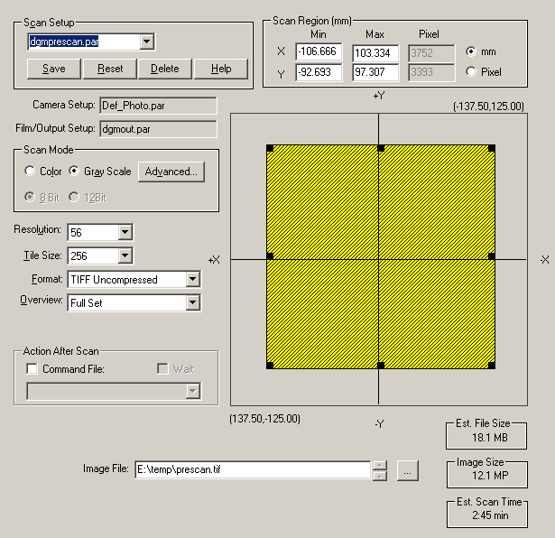
This page is used to set the area to scan (yellow area in the figure above), the pixel size (56 microns in the "Resolution" area of the figure), the mode (color vs gray, set in the example to "Gray Scale"), where to save the image collected during this scan (E:\temp\prescan.tif in this example). etc. The scan area can be altered by using the mouse (left button) to grab a black square in the corners or along the sides of the yellow area and dragging it appropriately.
Note that the "co-ordinate system" in this image i.e., the relationship of the scanned area to the platten area) is "left/right reversed." In other words, the upper left corner of any displayed scan is the upper right (relative to the rest of the scanned area) of the real platten as one looks at the scanner. This seems like a silly thing for PhotoScan to do, and one way to make it seem a bit less silly is to think of the images on the computer monitor as what one would see looking from below and through the glass plattens.
Always save images as "TIFF Uncompressed." For this overview scan, 56 micron pixels are fine. Any scans intended for data processing should be done at the highest possible resolution (7 microns) and binned appropriately at some later time. If one chooses not to scan using 7 micron pixels, note that all available pixels sizes are multiples of 7 microns. There should be preset parameter files (accessible through the "Scan Setup" area and called "dgmprescan.par" in this example) which will automatically set these prescan parameters properly.
- The second tab is the Film/Output page:
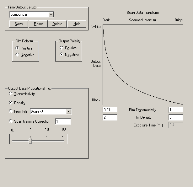
This page is used to set the film and output polarity (positive to negative in this example), the output data mode (set to density here) and the upper/lower limits for scanning (set here using Film Transmissivity from 0.01 to 1 or Film Density from 2 to 0). Film Transmissivity and Film Density are related by the following simple equation:
density = -log10( transmissivity ) and are coupled in the PhotoScan program (i.e., changing the density changes the transmissivity and vice versa). The PhotoScan program will not allow you to set improper limits (e.g., upper limits below lower limits).
The scanner will allow you to set a large Film Density range (e.g., 3 to 0), but the Zeiss only behaves well over approximately 1 OD unit (e.g., 1 to 0, 1.5 to 0.5, 2.0 to 1.0, etc.). Follow this link to see some data addressing this observation.
The "Film/Output Setup" area accesses stored parameter files (here that file is called "dgmout.par").
We have recently begun to scan using density mode and because we are using this mode, we also use either positive to negative or negative to positive polarity settings. The upper and lower limits will be reset for individual images (see the section below which deals with setting the histogram), but the range used in this example is a good starting point.
- Start the overview scan by clicking the "Start Scan" button
 in the menu bar.
NOTE: The scanner has been known to hang at this point. If that happens, turn the scanner off and back on, and allow the self-test to complete. Reboot the scanner's computer only after this has finished: the computer can be rebooted under conditions where it doesn't seem to know about the scanner, and if that happens, the machine must be rebooted again. Waiting until the self-test is complete guarantees that this will not happen.
- When a scan is done, a new window containing the scan appears. The initial view of the scanned area is "1:1 image pixel:monitor pixel" which means that one usually sees only a very small portion of the scanned image. The image can automatically be fit to the display region by first clicking on the "Fit Image" button
 in the menu bar and then clicking anywhere in the scan window.
- A typical overview of a single scanned micrograph looks like:
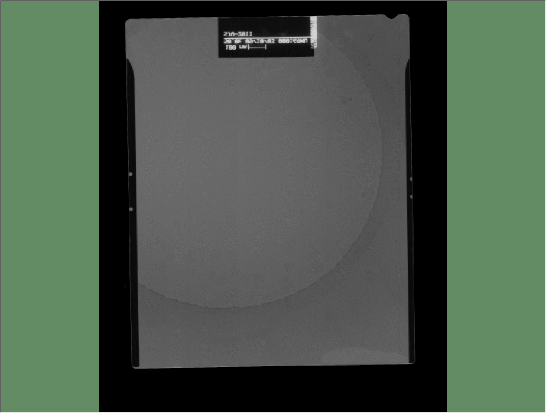
Note that in this display, the clear area of the micrograph which contains the date, magnification, etc. shows white text on a dark background. This is a consequence of using the positive to negative polarity settings mentioned earlier. This is the proper contrast for image processing here, and no operations that reverse this contrast are necessary (n.b., there may be circumstances where reversing this contrast is warranted, but those circumstances should be rare).
- Open the tabbed windows first seen in step 5 by clicking "File" -> "Scan Properties" in the menu bar. There is now a fourth tab (Histogram) which shows a histogram of the current scan:
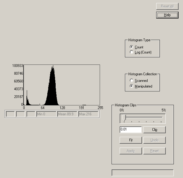
Switching from "Count" to "Log(Count)" in the "Histogram Type" box allows one to see the occupancy of infrequently used gray levels. For most practical purposes, the "Count" display is most informative. In the interests of truth in advertising, I must confess that I have no idea what the "Histogram Collection" box means or does. The "Histogram Clip" area allows the user to manipulate certain aspects of the histogram, but I do not know what such manipulations do nor whether they are useful.
Since this is the histogram of an overview scan, there is little to be gained by manipulating the scanner to change this: as long as the user can clearly see what should be scanned at higher resolution, the current scanner settings are fine.
- Use the stretchy box to select an area for a higher resolution scan. This can be accomplished either by manipulating the yellow scan area seen in step 5A above, or by clicking the
 button in the menu bar and drawing the stretchy box in the scan window directly:
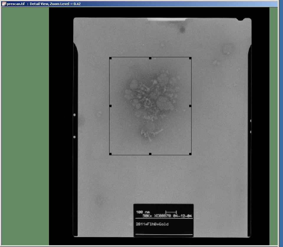
Also set the appropriate pixel size and both the file name and the location to save the high resolution scan (options in the Scan Setup tab). Save this information to a new parameter file ("Scan Setup" area in step 5A above).
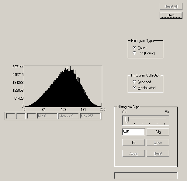
- At this point, it becomes important to set the upper and lower limits of the scanner appropriately. In the example above, the histogram of the overview indicates that most of the image data is compressed into a very narrow range of gray levels. A better image can be obtained by broadening the range of gray levels which contain most of the image data.
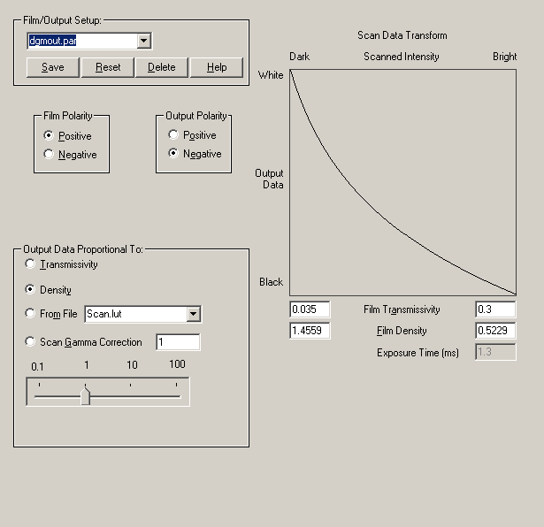
Since there is generally no need to scan the text window of a micrograph, it is possible to ignore the small peak at the left of the histogram (those few gray levels that describe the white text on a dark background) and to concentrate on spreading the more centrally located peak across all available gray levels. This is done by making adjustments to the "Film Transmissivity/Density" area of the "Film/Output" window. In a case like that illustrated above, it is necessary to bring the upper and lower limits much closer together.
This is the high resolution scan after performing this adjustment:
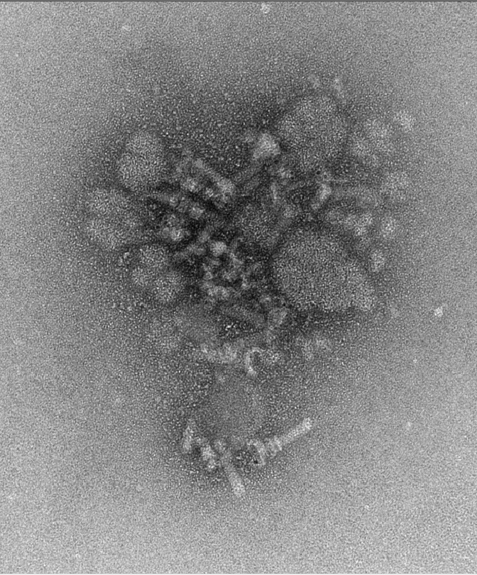
Here is the accompanying histogram, which is fully spread across all 256 gray levels:
In order to spread the histogram, the "Film Transmissivity" limits were changed from the initial 0.01 to 1.0 interval to the values shown here:
The process of adjusting the limits can be time consuming and will require practice to do well. The good news is that for a set of similar micrographs, the limits are likely to be similar if not identical.
- Changing the area to scan, the saved file's name and any adjustments to the scan limits is iterated until all the micrographs and areas have been scanned. At this point, power off the scanner and finish the entry in the log book. Remove negatives from the scanner and leave the scanner with a lint free cloth sandwiched between the glass plattens.
- The remaining step is to convert the scanned TIF files into MRC images. Start the conversion program by double clicking the
 icon on your desktop. This starts an easy to use program that looks like:
- Set the amount of averaging/binning in the "Pixel Averaging" area then drag all the images to be converted into the white panel below the "Apply Averaging" button. Click on the "All" button. This will start the conversion process, adding an "mrc" extension to the scanner file names (replacing the "tif" extension if it is used, or simply adding "mrc" to the file names if no extension was specified).
During the conversion, the user will see the program toggle between the input image and the (converted) output image. This comparison is shown in the following image pair:

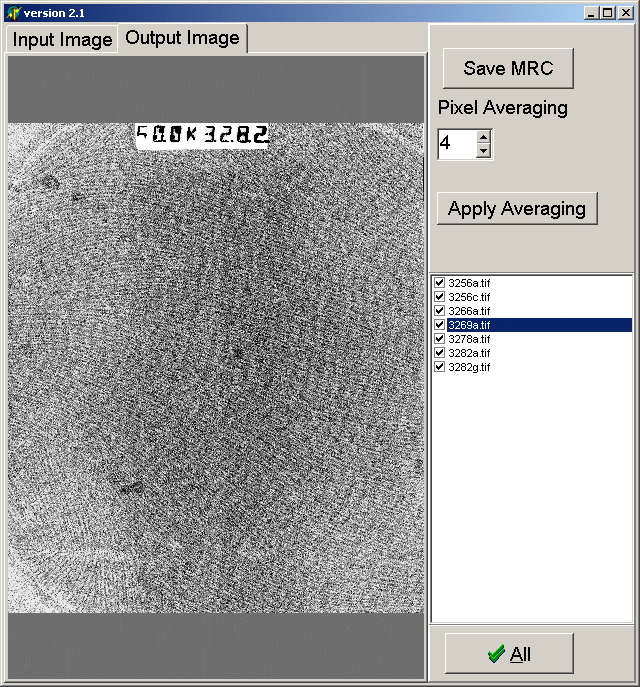
Note that there is no longer a contrast reversal between the input and output images. This is correct: the images were scanned in density mode and simply converted to MRC format (whereas previously the images were scanned in transmittance mode and transformed into density during the conversion to MRC format).

That's the short course in using the Zeiss scanner here at Brandeis.